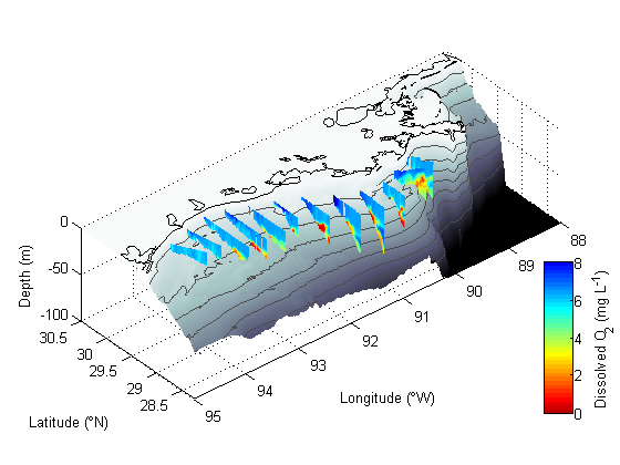
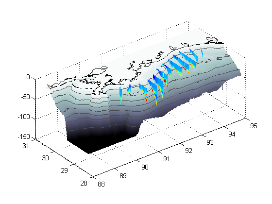
Making a map of nGOMEX region with curtain maps of oxygen

Contents

Example for MATLAB class

Part 0 - initializing the program

% Clear the workspace and close all open figure windows
clear
close all

% Here I'm defining variable names, the limits for the color axis and the
% string that we will use to label the colorbar. The variable name and
% label are cells, the color axis is a 1x2 array.
vars={'O2'};
cls=[0 8];
varn={'Dissolved O_2 (mg L^-^1)'};

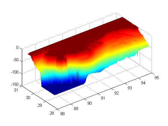
Part I - plot the bathymetry surface

The lines below load the bathymetry data I downloaded from NOAA, then adjust the values so that anything above the surface of the water is set to 0 and anything deeper than 100 m is set to 100 m. These are conventions purely for plotting.

load NGOMEX_seabathy_1min_NEW
depth(depth>=0)=0;
depth(depth<-100)=-100;

% These lines make a surface plot with the bathymetry, set the 'edgecolor'
% property of the surface to 'none', and set the aspect ratio of the plot
% based on a Mercator projection. The depth is shifted by 1.5 m purely to
% allow the contour lines (next part)
p=surf(-X,Y,depth-1.5);shading interp;hold on
set(p,'edgecolor','none')
set(gca,'dataaspectratio',[1 cos(nanmean(nanmean(Y'))*pi/180) 60]);
hold on

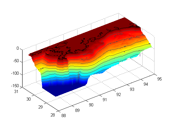
Part II - plot contour lines of certain isobaths

% Here we plot contour lines for certain isobaths, and shift these upward
% by slightly more than the surface. This allows these lines to sit on top
% of the surface plot so they are visible.  The loop below the countour
% call will set the colors of the contour lines by calling the individual
% handles for each line and setting the colors.
[c,ch]=contour3(-X,Y,depth-1,-80:10:-10,'k-');
for i=1:length(ch)
    set(ch(i),'color',[0.3 0.3 0.3]);
end

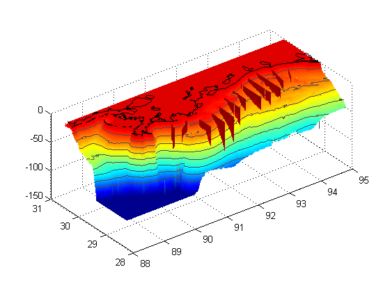
Part III - loading and plotting the coastline

% Here we load the coastline file, truncate it to fit in our plot, and then
% plot it as a dark black line.
load NGOMEXcoast
coast(coast(:,1)<-95 | coast(:,1)>-88 | ...
    coast(:,2)<28.25 |coast(:,2)>30.5 , :) =[];
plot(-coast(:,1),coast(:,2),'k-','linewidth',1);

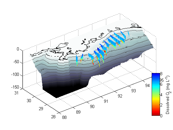
Part IV - curtain maps of the oxygen data.

% First we are setting up the different transect line names as a cell array
TRS={'B';'C';'D';'E';'Fa';'Fb';'G';'H';'J';'K';'Ia';'Ib';'W';'Q'};

% Here we loop through those transect line names...
for i=1:length(TRS);

    % ... and load them sequentially
    fname=['RAPID_2010_',TRS{i},'.mat'];
    load(fname);
    % The line below is left over from a previous version of this program
    % that cycled through not only the transect lines, but also different
    % variables, to plot various variables for each transect. Basically it
    % changes the variable name to "V".
    eval(['V=',vars{1},';']);
    V=-V;

    % Here we careate a surface plot of the data and set shading to interp
    surf(-X,Y,-Z,V)
    shading interp

    % Keep.m is a function I got from the file exchange that clears all
    % variables except those specified. Helpful to reduce memory useage
    % http://www.mathworks.com/matlabcentral/fileexchange/181-keep
    keep depth i TRS coast p c ch vars cls varn

end

Part V - Set the colors

% Setcolormaps.m is from the web and allows the use of two colormaps within
% one plot
% http://code.google.com/p/guillaumemaze/wiki/matlab_routines_setcolormaps
setcolormaps('bone','jet-1',-.000000001,512);

Part VI- the colorbar

% The lines below create a colorbar and then set various parameters for it
% including the axis limits, the y-label, and the position (which includes
% the size).
h=colorbar('location','eastoutside');

set(h,'clim',[0 512],'ylim',cls)
set(get(h,'ylabel'),'string',varn{1})
pos=get(h,'position');
pos(1)=pos(1).*1.07;pos(4)=pos(4).*0.4;
set(h,'position',pos);

Part VII - make it pretty

% These lines simply add axis titles, set axis limits, and rotate the
% figure to an aesthetically pleasing angle.
set(gca,'xdir','reverse')
xlabel('Longitude (\circW)');
ylabel('Latitude (\circN)');
zlabel('Depth (m)');

axis([88 95 28.25 30.5 -100 0])
view([-40 35])
shg

Published with MATLAB® 7.10