Contents

Model to show how small changes in survival affect population dynamics.

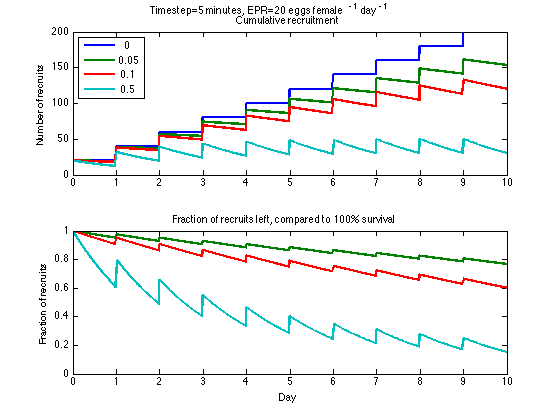
This simple model was developed to illustrate the implications for variable mortality rate on a population with a given growth rate. In this case that growth rate is assumed to be per capita egg production rate of a female, and does not include any mortality on the female. Thus, it is essentially a model of recruitment.

clear
days=10;
% Duration of the model run

eggs=20;
% Egg production rate (EPR)
% This is also the number of eggs we start with, and value for EPR.
% Each day the pop will increment by this value

Set up variables

% The following terms set up matrices in which we will put the results

timestep=5;
% This is the timestep - in minutes
deltat=timestep/(24*60);
% Puts the timestep in proper units (days)
death = [0 0.05 0.1 0.5];
% This sets the mortality rate on a per day basis

t=zeros(days/deltat,1);
% This will be my time variable
zoo=zeros(days/deltat,length(death));
% This tracks the population and goes into the plot
zoo(1,:)=eggs;
% setting the zero index as starting point

% initialize the counters to keep track of the results:
t(1)=0;
j=1;     % this is the counter to put stuff into whole spots in arrays
k=1;         % this counter keeps track of a whole day passing

Discrete Time Loop

for time=0:deltat:days          %This starts the cycle of days
    % checks if a day has passed so that eggs can be added into the
    % system once each day at midnight
    if k>=1/deltat
        zoo(j,:)=zoo(j-1,:)+eggs;
        % adding the eggs each day
        k=0; % reset the whole day counter
    end

    j=j+1;
    k=k+1;
    dailydeath = zoo(j-1,:).*(1-(exp(death.*deltat)));
    zoo(j,:)=zoo(j-1,:) + dailydeath;   %exponential calculation
    %zoo(j,:)=zoo(j-1,:)-zoo(j-1,:).*deltat.*death;   %THIS GIVES THE SAME RESULT!!
    t(j)=time;

end

Plot the Results

figure
subplot(2,1,1)
plot(t(1:j-3,:),zoo(1:j-3,:),'linewidth',2)
title(['Cumulative recruitment'])
set(gca,'xtick',[0:days])
ylabel('Number of recruits')
legend([num2str(death')],2)
% text(1.15,(.9*max(ylim)),['Final Recruitment (Day ',num2str(days/2),')  =',num2str(round(zoo((j/2-3),:))) ])
% text(2.15,(.8*max(ylim)),['Recruitment (Day ',num2str(days),')  =',num2str(round(zoo((j-3),:))) ])
% text(2.25,(.8*max(ylim)),'N_t = N_0\ite\rm^(^-\it^m^ ^t\rm^)')

for i=1:length(death)
    zoop(:,i)=(abs(zoo(1:j,i))./zoo(1:j,1));
end

subplot(2,1,2)
plot(t(1:j-3,:),zoop(1:j-3,:),'linewidth',2)
set(gca,'xtick',[0:days])
ylim([0 1])
% legend([num2str(death')],3);
title(['Fraction of recruits left, compared to 100% survival']);
% text(0.15,.2,['% Recruits (Day ',num2str(days/2),')  =',num2str((round(zoop((j-3),:).*100))./100) ])
% text(1.15,.1,['% Recruits (Day ',num2str(days),')  =',num2str((round(zoop((j/2-3),:).*100))./100) ])
xlabel('Day')
ylabel('Fraction of recruits')

[ax,h]=suplabel(['Timestep=',num2str(timestep),' minutes, EPR=',...
    num2str(eggs),' eggs female^-^1 day^-^1'],'t');

Published with MATLAB® 7.13